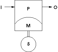
Recall our input/output model of a computer, consisting of a processor or CPU (P), (volatile) memory (M), input (I), output (O) and pervasive storage (S):
Pretty much every computer looks like this model at some high level of abstraction. And, at the lowest level of abstraction, every computer is simply manipulating bits or sets of bits. So the real question is how do things organize ``inside the box'' above and on down to the bit level? Your book spends some time trying to fill in this middle ground, with gates and devices like registers, adders, and so on. We're going to skip much of this detail and jump up one (very big) step to the register level to see one model of what's inside the processor/memory box. Of course, there are lots of ways to skin this cat, and your book, in Chapter 5, describes another machine that is somewhat more complicated than this one, but that shares nearly all of the features described here (they are, in fact, more similar than dissimilar, which is pretty much the case for most such machines). You should of course feel free to read about the Chapter 5 architecture, but I prefer to talk about this architecture in class because its quite a bit simpler yet still sufficient to give you a good picture of what goes on inside the machine.
Our model is an example of an architecture called a "one address machine," so we'll call our machine the OAM. Our machine is quite simple, but has the same basic functionality you will find in a real machine: it will follow the instructions given in programs we write, reading inputs as needed from the keyboard and writing output as directed to the screen of our hypothetical machine.
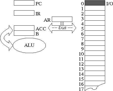
Our machine consists of some memory, a controller or control unit which contains a few extra memory locations and manages the operation of the machine, and an arithmetic-logic unit or ALU which performs the basic arithmetic and logical operations for our simple computer (see figure).
You can think of the OAM's memory like the letterboxes behind a hotel desk. Each memory location is identified with an address, where the lowest address is 1 and each subsequent letterbox is numbered consecutively. In principle, each memory location might contain any type of data, provided it has enough bits to hold the representation of the intended datum (in a real machine, each memory location consists of a fixed number of bits, generally 32 or 64, which correspond to the word length of the machine). Here, we'll make a sweeping simplifying assumption that each memory location is large enough to contain any single datum, without regard to how large the datum really is in terms of the number of bits required to store its representation. As a second, equally sweeping, simplifying assumption, we will consider the OAM's memory to be infinitely large. Naturally, that's sort of silly; real computers have limited amounts of memory to hold programs and data. But since our programs will be small, it's OK to assume memory is infinite (we'll ignore storage altogether; once you have infinite amounts of memory, who's counting?).
The control unit also contains five additional memory locations called registers. The five registers, labeled PC (program counter), IR (instruction register), AR (address register), ACC (accumulator), and B (b register), are used to manage the operation of the control unit, including its interaction with memory. Each register has a specific function, which is implied by its name, and which will become clear as we study the operation of the OAM.
Once the OAM is turned on, the control unit follows a fixed sequence of operations called the instruction cycle. As the name implies, the instruction cycle repeats forever, or at least until the OAM is turned off. The instruction cycle consists of three distinct phases: a fetch phase, an increment phase, and an execute phase. During each of these phases, the control unit interacts with the appropriate registers and, possibly, with memory, to perform the appropriate calculations as goverened by the program we give to the OAM.
Our program, written in OAM machine language, resides in memory starting at a known designated address. Here we'll adopt the convention that programs are always stored beginning in memory location 1. At the machine level, the program consists of a set of instructions written in a fully-specified language that the OAM can understand, and not in a higher-level programming language like Python, C, C++, Java or Perl. Indeed, programs written in such higher-level languages must first be translated into OAM machine language if we intend to run them on our machine.
For our OAM example, the language contains only 16 different instructions. The specification of these instructions, called the instruction set architecture, is generally the first step computer engineers take when designing a new computer; the instruction set architecture fully describes the functionality of the machine, and is specific to this particular machine design. OAM instructions manipulate the computer's memory, registers, ALU, and input/output facilities. Machine language programs are directly executed by the control unit, with no further need for interpretation.
The fetch-increment-execute cycle governs the behavior of the machine as it performs the instructions specified in the program. In the fetch phase, the "next" OAM instruction to execute is copied from memory to the control unit's instruction register (IR). What determes which instruction is "next" to execute is the value of the program counter (PC). When we first turn the machine on, the PC is initialized to 1, in concordance with our convention that the program we are executing is stored in memory starting with memory location 1. During the increment phase, the value in the program counter is increased by 1, meaning that the "next" instruction to execute can be found in memory location 2, then 3, and so on. The increment phase enforces the convention that the instructions in our OAM program are by default executed sequentially: our machine deviates from this default convention only under explicit program control, as we will describe later.
The execute phase is the most complex part of the instruction cycle. What actually occurs during the execute phase is dependent on the contents of the IR. Depending on the OAM instruction we are executing, different changes in the machine's state will occur. For example, some instructions will cause new values to be written to memory, or cause certain arithmetic operations to take place in the ALU. The execute phase of the instruction cycle is therefore where any actual computation takes place.
The fetch-increment-execute cycle repeats until the program orders the machine to halt; we'll get back to exactly how it works in more detail just a bit later.
The instruction set is the collection of lowest-level commands the computer is able to execute. The instruction set design is heavily influenced by the underlying computer architecture, because the semantics of each instruction can be defined by the changes it causes in the machine's internal state. It is the responsibility of the controller to interpret an instruction, telling the other parts of the computer what to do.
Our instruction set is pretty simple by modern standards, having only a handful of instructions. Each instruction consists of at most two parts, an operation code (or opcode) and a single (optional) operand, (usually a memory address; hence, the name "one address machine"). Usually, each instruction is stored in a fixed number of bits, with a certain agreed-upon number of bits dedicated to opcode and a certain agreed-upon number of bits dedicated to operand, where the number of bits devoted to each is part of the instruction set design and restricts, e.g., the amount of memory the machine can utilize, or the number of different instructions in the instruction set.
The ALU instructions are those instructions that direct the arithmetic-logic unit to perform actual calculations. OAM ALU instructions operate on the B register and the accumulator, or ACC. In every case, the instruction operand corresponds to a memory address: the OAM first copies the contents of the memory address specified by the operand into the B register, performs whatever operation is specified by the operator, and stores the result in the ACC, overwriting whatever was there in the first place.
The ALU instructions are (for convenience we will be using 3-letter mnemonic forms for each operator rather than the binary opcode typically associated with each operator internally):
ADD address     # load B, add ACC and B, store result in ACC
SUB address     # load B, subtract B from ACC, store result in ACC
MLT address     # load B, multiply ACC and B, store result in ACC
DIV address     # load B, divide ACC by B, store result in ACC
All of these are binary instructions that operate on both the ACC and the B register. Note that our ALU commands really only control the arithmetic part of the ALU; there are no logical commands such as OR, AND or NOT which one would find on a real computer. That's OK for now, since we'll only be dealing with integer operations in our examples; in a real computer, we'd have some additional logical operands.
In addition, we have four additional ALU instructions that do not interact with memory:
SET value       # set ACC to value
NEG             # negate ACC
INC             # increment ACC value by 1
DEC             # decrement ACC value by 1
These operations can be used to manipulate the contents of ACC directly.
Next, we'll need some memory manipulation instructions for the OAM. The basic operations we need to perform on the memory are to fetch the contents of a specified memory address and to write something back into a specified memory location. We'll adopt the convention that all interaction between the ALU and the memory occurs through the ACC register. Memory instructions are also one-address instructions, where the operand corresponds to the memory location we're reading from or writing to. Thus:
LDA address      # load ACC with value stored in specified memory location
STA address      # store contents of ACC in specified memory location.
As well as memory, OAM needs to be able to read from the computer's input devices (e.g., the keyboard) and write to the computer's output devices (e.g., the screen). For simplicity, the OAM will use a special technique that treats I/O (or input/output) as memory operations on special addresses. We'll distinguish the special memory address 0 as the I/O address; any LDA or STA operations on location 0 will correspond to reading from input or writing to output, respectively. This technique is very similar to what is often called memory-mapped I/O.
OAM executes each instruction in the program and goes on to the next instruction. Some instructions, however, are used to alter the flow of control from this sequential model. We call these control instructions branch instructions; they come in two flavors, conditional and unconditional. The unconditional branch is a one-address instruction that instructs the computer to "take the next instruction from memory location address instead of current address +1."
BR address # take next instruction from addressBR operates by placing its argument directly in the PC, overwriting whatever value was there.
The conditional branches are a bit more complex. They need to be able to test a condition and determine where to take the next instruction from. The OAM has two conditional branch instructions, BRZ and BRP, which test the value stored in ACC to decide whether or not to branch:
BRP address     # next instruction from address if ACC is positive, else ignore
BRZ address     # next instruction from address if ACC is zero, else ignore
In other words, BRP branches to the specified instruction only if ACC is positive, while BRZ branches only if ACC is zero. If the condition isn't met, then the next instruction is taken from the regular place. There are two additional branch instructions, BRI, or "branch indirect," and BRS, or "branch and store," which will be described in more depth later.
Finally, we'll need an instruction to tell OAM when the program is finished.
HLT # stop OAMNote that the HLT instruction has no operand.
Before we go into more detail about the fetch-increment-execute behavior of the controller, let's look at a sample machine language program for the OAM. This program computes the value of the expression (A+B)^2 where A and B are read in from the keyboard, in that order (note: we'll use ^ to represent exponentiation). The result is written out to the screen. Note that we're careful not to store our values in a memory location that might conflict with the program itself.
1. LDA 0                  # read in value of A from keyboard
2. STA 100                # store it in memory location 100
3. LDA 0                  # read in value of B from keyboard
4. ADD 100                # add A to B
5. STA 100                # store A+B in memory location 100
6. MLT 100                # multiply A+B by itself
7. STA 0                  # write ( A + B ) ^ 2 to screen
8. HLT                    # halt
Before we examine the program more closely, there are a few conventions we need to establish. First, while we'll start each line with a consecutive line number to facilitate our discussion, the line number itself is not a part of the program, and should be considered optional. Second, we'll use the convention that any words that follow the special character "#" are ignored by the one address machine; they are only there for us to make notes to help the reader understand the program.
It takes 8 instructions just to compute and print the value of this expression! That's because machine language instructions are at the very lowest level of computer design; they specify very tiny aspects of a computer's operation. Thus, machine language programs tend to be longer than what you might expect.
Here's an OAM program for use by NASA that counts down from 10 to 1, printing out each number on the screen. Note the use of the BRP instruction.
1. SET 10               # set ACC to 10
2. STA 0                # write out number in ACC
3. DEC                  # decrement by 1
4. BRP 2                # are we done yet? else go to step 2
5. HLT                  # halt
Let's examine in more detail how the OAM operates. Note that the program is loaded into memory starting by convention in memory location 1. We'll show how the OAM operates by giving you snapshots of the OAM's internal state; in other words, just what the registers inside the machine contain at a given time. The initial state of the OAM looks like:
PC=1; AR=?; IR=?; ACC=?; B=?Note that we don't really know what some of the registers contain initially; our only guarantee is that PC will point to memory location 1, which is where we've established the program should start.
Next we'll emulate the fetch-increment-execute cycle of the OAM. The fetch phase of the cycle copies the contents of the PC to the AR, and then reads the memory location specified by the AR value into the IR. This is called a fetch since we are in essence fetching the next program instruction into the IR. The state of the OAM is now:
PC=1; AR=1; IR=SET 10; ACC=?; B=?The increment phase of the cycle is simple; the PC's value is simply incremented by 1 and then the whole cycle is repeated.
PC=2; AR=1; IR=SET 10; ACC=?; B=?The next phase is the execute phase. It is here that the OAM actually does what it's instructed to do by the contents of the IR. Since each instruction has a different meaning, exactly what the OAM does here also differs for each instruction. For the SET instruction, the operand is simply copied into the ACC:
PC=2; AR=1; IR=SET 10; ACC=10; B=?
Note that for more complex instructions that require interaction with memory, such as ADD, the OAM would copy the operand into the AR, fetch the value of memory at the location specified by the contents of the AR into the B register, and perform the addition, leaving the result in the ACC.
Consider the following somewhat nonsensical OAM program:
1.  LDA 0
2.  STA 5
3.  INC
4.  BR  6
5.  DEC
6.  LDA 0
7.  MLT 5
8.  STA 0
9.  DEC
10. BRZ 12
11. BR  8
12. HLT
Assume any inputs required by the program are taken, in order, from the input sequence {2, 2, 4, 4, 6, 6, ...}. What output, if any, would you observe as this program is executed? Also, what is left in each of the registers (PC, IR, AR, ACC, and B) once the program halts? Finally, how would the program's behavior differ if statement 11 read BR 9 instead?
We can extend the basic OAM instruction set with just a few additional instructions to significantly enhance its capabilities.
The first advanced instructions, mentioned previously, are the branch indirect and branch and store instructions.
BRI address     # next instruction from address stored in address
BRS address     # next instruction from address+1, store current PC in address
The BRI instruction is nearly identical to to the unconditional branch instruction BR, except that the next instruction is not taken from the stated address, but, rather from the address stored in that address. This added level of indirection allows us to use a series of OAM instructions to calculate an address to which we wish to branch. By placing the calculated address in a memory location and then issuing a BRI, we are essentially allowing the program to modify its own execution. All architectures support some form of this important concept.
The BRS instruction is also essentially an unconditional branch instruction. But unlike the standard unconditional branch, the branch and store "remembers" where it came from by storing the current PC value in memory at the branch address (the next instruction is then read from the memory location after the branch address).
We can use the BRS and BRI instructions together to construct a program segment that can be shared and reused many times within the same program. For example, let's assume we are writing a program that requires us to compute the square root of several numbers. Since the OAM instruction set does not directly support square root calculations, we'll need to write a little OAM program that calculates the square root using only OAM instructions; while this isn't necessarily difficult, it does require a sequence of some number of OAM instructions.
Since we'll be computing square roots many times, it makes sense to write the square root "subprogram" only once, and then "use" or "invoke" it whenever we need to compute a square root. Such program fragments are called subroutines; we "invoke" or "call" a subroutine, perform whatever calculation it encodes, and then go back or "return" to whatever we were doing when we called the subroutine.
The BRS and BRI instructions, when used together, yield a rudimentary mechanism for creating subroutines. While somewhat limited, this is an adequate example of how this kind of thing might be accomplished in a real architecture, even if real machines ultimately require a more robust and concomitantly more complex mechanism.
An example should help make this idea clear. Consider the following OAM program, with the instructions in steps 7-9 constituting a subroutine that adds 1 to whatever value is currently in the the accumulator.
1. LDA 0
2. BRS 7
3. BRS 7
4. BRS 7
5. STA 0
6. HLT
7. NOOP
8. INC
9. BRI 7
What does this program produce on the screen? (Answer: whatever number is read from the keyboard, plus 3.)
Ignoring for now the (new) NOOP instruction in step 7, consider that, once the OAM initializes the accumulator to whatever value is read from the keyboard in step 1, the BRS in step 2 stores the current PC value (3) in memory location 7 and resumes execution at step 8. The BRI in step 9 reads the value stored in location 7 by the BRS and forces the OAM to take its next instruction from this location (3). The same call/return sequence occurs three times, with each successive BRS storing a different value in memory location 7, which causes the BRI to resume processing at the instruction following the BRS that invoked the subroutine.
So what is this NOOP instruction? The NOOP, or "no operation," is not really an instruction; it's just a placeholder that helps us to recognize that (1) that particular memory location is not an executable instruction but rather (2) will be overwritten by something else in due course. Here, the something else is the subroutine's return address. Notice how convenient the use of indirect addressing is in this situation: we ensure our OAM program does the appropriate calculation, leaving an appropriate address value in memory location 7, and then we use the BRI to simply "go there."
BRI is an example of an entire class of instructions that use indirect addressing. Many real machines offer, for example, indirect arithmetic operations which are to their vanilla form as BRI is to BR. For example, consider a hypothetical ADDI instruction, which adds to the accumulator the value stored at the location stored in the specified address. Such an instruction could be very useful if we were, say, interested in adding together some number of consecutive memory locations. In such a situation, we could simply load the accumulator with the value stored in the first of these memory locations, and then execute repeated ADDI instructions alternating with an INC to increment the value stored at the ADDI address.
We don't choose to include additional indirect addressing instructions in our OAM because there are other ways to achieve the same effect, even if they are perhaps somewhat less convenient to use. As always, designing an artifact like a computer involves making a whole set of decisions, which typically trade off one factor (e.g., size and complexity of the instruction set) against another factor (e.g., ease of use).
It should be readily apparent that machine language programming is at best tedious, and can also be enormously difficult. Consider what happens, for example, if one wanted to alter the previous example so that four consecutive subroutine invocations were to be made rather than just three. But simply inserting an additional BRS instruction won't solve my problem, because the relocation of the instructions that follow the additional BRS require making changes to the layout of the instructions in memory. The corrected program would then be:
1. LDA 0
2. BRS 8
3. BRS 8
4. BRS 8
5. BRS 8
6. STA 0
7. HLT
8. NOOP
9. INC
10. BRI 8
The problem here is that the mapping of the program to memory locations in the OAM must be done manually by the programmer. Any change in instruction location may require changes to addresses throughout the program. Unfortunately, determining exactly which values must be changed because of relocation isn't necessarily easy. In this example, every 7 became an 8, but that's not necessarily the case for every program. Imagine a program that not only used the numebr 7 as an address, but also contained an explicit SET 7 instruction in the course of its calculation. Changing this 7 would surely have unintended effects on the computation, and having to make these corrections manually may well introduce all sorts of extraneous errors which are hard to track and correct (missing a value that should have been changed, or changing a value that shouldn't have been changed).
Fortunately, there is a way to alleviate these kinds of bothersome bookkeeping issues. Computers are very good at bookkeeping, much better than people are. So why not write a computer program to help minimize the tediousness of machine language programming?
One such program is called an assembler. An assembler is a simple language translator, that takes as input a program in one language and outputs a program in another. Here, the input language is the OAM assembly language, and the output language is our familiar OAM machine language. These two languages don't really differ much: mostly, the OAM assembler allows us to use symbolic names for, e.g., memory locations rather than have to keep track of all of the addresses ourseleves.
In fact, up to now, we've been cheating just a bit and have been using a feature typical of assemblers in our discussion of machine language. A real machine language program doesn't use 3-letter mnemonic codes for instructions in the instruction set; instead, it uses binary opcodes, or simply patterns of 1's and 0's, to stand in for each instruction. In assembly language, use of mnemonic opcodes is the norm; the assembler simply translates our 3-letter code into the appropriate bit pattern.
In a similar vein, our OAM assembler supports the use of address labels rather than using explicit memory addresses. An example should help make this clear. Recall our subroutine example, now rewritten using labels (which appear at the beginning of a line, followed by a comma):
1.        LDA 0
2.        BRS MyInc
3.        BRS MyInc
4.        BRS MyInc
5.        STA 0
6.        HLT
7. MyInc, NOOP
8.        INC
9.        BRI MyInc
The use of a label for the subroutine not only makes the subrouting independent of explicit memory addresses (so that it can be shifted around a bit in memory as the program is modified), but it also allows the programmer to give a more meaningful, mnemonic, name to the subroutine.
We can extend this idea just a little bit further to make our assembly language code still more readable. Recall our use of the special memory location 0 to stand for reading from input (in the case of LDA) or writing to output (in the case of STA). By defining two special labels "stdin" and "stdout" (for "standard input" and "standard output") to always correspond to memory location 0, we can rewrite our program as:
1.        LDA stdin
2.        BRS MyInc
3.        BRS MyInc
4.        BRS MyInc
5.        STA stdout
6.        HLT
7. MyInc, NOOP
8.        INC
9.        BRI MyInc
which is not only much more readable than the original program shown above, but is likely to be more easily modified without introducing spurious errors.
Let's look at another example of OAM assembly language programming. Assume we're interested in checking a number, let's call it X, which is provided as input, to see if it is prime (recall a prime number is a whole number greater than 1 that can only be divided by 1 and itself; the first few prime numbers are 2, 3, 5, 7, 11 and 13). One way of doing so is to try dividing X by all possible numbers from 2 up to the square root of X: if any of these numbers divide X exactly, then X cannot be prime. Our OAM program will print "composite" if the number is not prime and "prime" if the number is prime.
Note that this isn't by any stretch of the imagination the best or most efficient way of checking a number for primality, but it is a simple solution that provides a good OAM program example of some sophistication.
We'll develop our program in several stages. Here, as before, we'll number the lines in order to be able to more easily refer to particular instructions in our discussion: the line number itself is optional and should not be considered a part of the program. Also, we'll continue to use the symbol # to indicate that the remainder of the line can be ignored: this is a useful trick so that we can document what our program is doing for a human reader along with the OAM instructions.
First, we'll read the number we're testing for primality in from the standard input (memory location 0), and store the value in an appropriate memory location (label x).
1.        LDA stdin     # Read in candidate number
2.        STA X         # Store in memory location labeled x
Since the smallest prime number is 2, anything less than 2 cannot be prime. Let's rule the simple cases out first.
3.        SET 2         # Set the accumulator to 2
4.        SUB x         # ACC = 2-x
5.        NEG           # ACC = x-2
6.        BRZ true      # x=2 is prime
7.        BRP more      # x>2 continue checking
8. false, SET composite # not prime, print "composite"
9.        STA stdout
10.       HLT
11. true, SET prime     # prime, print "prime"
12.       STA stdout
13.       HLT
There are two unusual things going on here. First, notice the use of two almost-subroutines at labels false and true. These differ from the subroutines we've seen before in that they are simply labels we branch to with BR, BRZ, or BRP instructions rather than labels branced to with a BRS instruction. They are different because here we have no expectation of ever "returning" from the subroutine: instead, once we branch to the appropriate label, the program is guaranteed to halt after just a few additional steps, which simply produce the appropriate output before terminating the program.
The second unusual thing occurs in lines 8 and 11. Up to this point, we've only allowed numbers to be stored in memory locations, not strings of characters like "composite" or "prime." But as you may recall, we originally said we would assume that each OAM memory location is large enough to contain any single datum, so here we're allowing the character strings "composite" and "prime" to be stored in a single memory location, in this case, the standard output. This allows us to print more meaningful messages to the output.
At this point, we know that the number is greater than 2. So we continue by "testing" the candidate prime by dividing it by 2, then by 3, and so on, all the way up to the first quotient that exceeds the square root of the candidate prime. If any of these quotients divide the candidate exactly, then the candidate can not be prime. On the other hand, if we reach the square root of x without finding any number that exactly divides X, then X must be prime. Here's how that code looks:
14. more, SET 2                 # Start checking for division by 2
15. loop, STA q                 # Store quotient in q
16.       BRS check             # Jump to integral division check
17.       LDA q                 # Are we done?
18.       MLT q
19.       SUB x                 # If q^2 > x, then we're done
20.       BRP true              # Must be prime to have survived
21.       LDA q
22.       INC                   # Else, increment q and repeat
23.       BR loop
Note the structure of the code: we continue to loop through instructions 15 through 23, incrementing the quotient q (which starts at 2) by one each time and checking for exact division using the check subroutine (see below). When q^2 exceeds x, we know we've survived all possible checks, so we branch to the true label, which prints out "prime" and halts the program.
The only thing that remains to write is the check subroutine. This subroutine needs to check x for exact division by q; exact division means that the whole number part of (x / q) times q must equal exactly x (in other words, (x / q) has remainder 0). Lacking any elegant means to extract only the whole number part of a division, we'll resort to a less elegant and much less efficient mechanism: division by repeated subtraction.
The idea is that to check if q divides x exactly, it is sufficient to repeatedly subtract q from x until either x goes to 0 (in which case, q divides x exactly) or x is less than 0 (in which case q does not divide x exactly).
24.check, NOOP                  # Integral division check subroutine
25.       LDA x                 # ACC = x
26.  sub, SUB q                 # ACC = ACC - q
27.       BRZ false             # q divides x exactly
28.       BRP sub               # Keep subtracting q
29.       BRI check             # Return, q fails to divide x
Finally, we need to make sure we have lables corresponding to the memory locations needed to store and values we've used in the program, here x and q.
30. x,    NOOP                  # Candidate prime number from stdin
31. q,    NOOP                  # Candidate quotient
That's it. The whole program takes 31 memory locations, although the exact structure of the program could be manipulated a bit without changing the basic design, by, for example, shuffling the order of the subroutines.
Those of you who are intrigued by this sort of thing might consider following up with one of the following two items:
Soul of a New Machine, Tracy Kidder (1981).
The Cartoon Guide to Computer Science, Larry Gonick (1983).
The Kidder book in particular is quite readable, while the Gonick book is pretty entertaining.